扩散模型之DDIM

Author: [小小将]

Link: [https://zhuanlan.zhihu.com/p/565698027]

“What I cannot create, I do not understand.” -- Richard Feynman

上一篇文章https://zhuanlan.zhihu.com/p/563661713 (opens new window)介绍了经典扩散模型DDPM的原理和实现，对于扩散模型来说，一个最大的缺点是需要设置较长的扩散步数才能得到好的效果，这导致了生成样本的速度较慢，比如扩散步数为1000的话，那么生成一个样本就要模型推理1000次。这篇文章我们将介绍另外一种扩散模型DDIM（https://arxiv.org/abs/2010.02502 (opens new window)），DDIM和DDPM有相同的训练目标，但是它不再限制扩散过程必须是一个马尔卡夫链，这使得DDIM可以采用更小的采样步数来加速生成过程，DDIM的另外是一个特点是从一个随机噪音生成样本的过程是一个确定的过程（中间没有加入随机噪音）。

DDIM原理

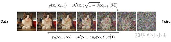
在介绍DDIM之前，先来回顾一下DDPM。在DDPM中，扩散过程（前向过程）定义为一个马尔卡夫链：

$q({\mathbf{x}}_{1:T}|{\mathbf{x}}_0)=\prod _{t=1}^{T}q({\mathbf{x}}_t|{\mathbf{x}}_{t-1})q({\mathbf{x}}_t|{\mathbf{x}}_{t-1})=\mathcal{N}({\mathbf{x}}_t;\sqrt{\frac{{\alpha }_t}{{\alpha }_{t-1}}}{\mathbf{x}}_{t-1},(1-\frac{{\alpha }_t}{{\alpha }_{t-1}})\mathbf{I})$

注意，在DDIM的论文中，${\alpha }_t$ 实是DDPM论文中的${\overline{\alpha }}_t$，那么DDPM论文中的前向过程${\beta }_t$ 为：

${\beta }_t=(1-\frac{{\alpha }_t}{{\alpha }_{t-1}})$

扩散过程的一个重要特性是可以直接用${\mathbf{x}}_0$ 对任意的${\mathbf{x}}_t$ 行采样：

$q({\mathbf{x}}_t|{\mathbf{x}}_0)=\mathcal{N}({\mathbf{x}}_t;\sqrt{{\alpha }_t}{\mathbf{x}}_0,(1-{\alpha }_t)\mathbf{I})$

而DDPM的反向过程也定义为一个马尔卡夫链：

$p_{\theta }({\mathbf{x}}_{0:T})=p({\mathbf{x}}_T)\prod _{t=1}^T{p}_{\theta }({\mathbf{x}}_{t-1}|{\mathbf{x}}_t)p_{\theta }({\mathbf{x}}_{t-1}|{\mathbf{x}}_t)=\mathcal{N}({\mathbf{x}}_{t-1};{\mathit{\mu }}_{\theta }({\mathbf{x}}_t,t),{\mathbf{\Sigma }}_{\theta }({\mathbf{x}}_t,t))$

这里用神经网络$p_{\theta }({\mathbf{x}}_{t-1}|{\mathbf{x}}_t)$ 拟合真实的分布$q({\mathbf{x}}_{t-1}|{\mathbf{x}}_t)$。DDPM的前向过程和反向过程如下所示：

我们近一步发现后验分布$q({\mathbf{x}}_{t-1}|{\mathbf{x}}_t,{\mathbf{x}}_0)$ 一个可获取的高斯分布：

$q({\mathbf{x}}_{t-1}|{\mathbf{x}}_t,{\mathbf{x}}_0)=\mathcal{N}({\mathbf{x}}_{t-1};\tilde{\mathit{\mu }}({\mathbf{x}}_t,{\mathbf{x}}_0),{\tilde{\beta }}_t\mathbf{I})$

其中这个高斯分布的方差是定值，而均值是一个依赖${\mathbf{x}}_0$ ${\mathbf{x}}_t$ 组合函数：

${\tilde{\mathit{\mu }}}_t({\mathbf{x}}_t,{\mathbf{x}}_0)=\frac{\sqrt{{\alpha }_t}(1-{\alpha }_{t-1})}{\sqrt{{\alpha }_{t-1}}(1-{\alpha }_t)}{\mathbf{x}}_t+\frac{\sqrt{{\alpha }_{t-1}}{\beta }_t}{1-{\alpha }_t}{\mathbf{x}}_0$

然后我们基于变分法得到如下的优化目标：

$\begin{array}{rl}L& ={\mathbb{E}}_{q({\mathbf{x}}_{1:T}|{\mathbf{x}}_0)}[\log \frac{q({\mathbf{x}}_{1:T}|{\mathbf{x}}_0)}{p_{\theta }({\mathbf{x}}_{0:T})}]\\ & =\underset{L_T}{\underbrace{D_{\text{KL}}(q({\mathbf{x}}_T|{\mathbf{x}}_0)\parallel p_{\theta }({\mathbf{x}}_T))}}+\sum _{t=2}^T\underset{L_{t-1}}{\underbrace{{\mathbb{E}}_{q({\mathbf{x}}_t|{\mathbf{x}}_0)}[D_{\text{KL}}(q({\mathbf{x}}_{t-1}|{\mathbf{x}}_t,{\mathbf{x}}_0)\parallel p_{\theta }({\mathbf{x}}_{t-1}|{\mathbf{x}}_t))]}}-\underset{L_0}{\underbrace{{\mathbb{E}}_{q({\mathbf{x}}_1|{\mathbf{x}}_0)}\log p_{\theta }({\mathbf{x}}_0|{\mathbf{x}}_1)}}\end{array}$

根据两个高斯分布的KL公式，我们近一步得到：

$L_{t-1}={\mathbb{E}}_{q({\mathbf{x}}_t|{\mathbf{x}}_0)}[\frac{1}{2{\sigma }_t^2}\parallel {\tilde{\mathit{\mu }}}_t({\mathbf{x}}_t,{\mathbf{x}}_0)-{\mathit{\mu }}_{\theta }({\mathbf{x}}_t,t){\parallel }^2]$

根据扩散过程的特性，我们通过重参数化可以近一步简化上述目标：

$L_{t-1}={\mathbb{E}}_{{\mathbf{x}}_0,ϵ\sim \mathcal{N}(\mathbf{0},\mathbf{I})}[\frac{{\beta }_t^2}{2{\sigma }_t^2{\alpha }_t(1-{\overline{\alpha }}_t)}\parallel ϵ-{ϵ}_{\theta }(\sqrt{{\overline{\alpha }}_t}{\mathbf{x}}_0+\sqrt{1-{\overline{\alpha }}_t}ϵ,t){\parallel }^2]$

如果去掉系数，那么就能得到更简化的优化目标：

$L_{t-1}^{\text{simple}}={\mathbb{E}}_{{\mathbf{x}}_0,ϵ\sim \mathcal{N}(\mathbf{0},\mathbf{I})}[\parallel ϵ-{ϵ}_{\theta }(\sqrt{{\overline{\alpha }}_t}{\mathbf{x}}_0+\sqrt{1-{\overline{\alpha }}_t}ϵ,t){\parallel }^2]$

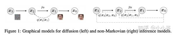
仔细分析DDPM的优化目标会发现，DDPM其实仅仅依赖边缘分布$q({\mathbf{x}}_t|{\mathbf{x}}_0)$，而并不是直接作用在联合分布$q({\mathbf{x}}_{1:T}|{\mathbf{x}}_0)$。这带来的一个启示是：DDPM这个隐变量模型可以有很多推理分布来选择，只要推理分布满足边缘分布条件（扩散过程的特性）即可，而且这些推理过程并不一定要是马尔卡夫链。但值得注意的一个点是，我们要得到DDPM的优化目标，还需要知道分布$q({\mathbf{x}}_{t-1}|{\mathbf{x}}_t,{\mathbf{x}}_0)$，之前我们在根据贝叶斯公式推导这个分布时是知道分布$q({\mathbf{x}}_t|{\mathbf{x}}_{t-1})$ ，而且依赖了前向过程的马尔卡夫链特性。如果要解除对前向过程的依赖，那么我们就需要直接定义这个分布$q({\mathbf{x}}_{t-1}|{\mathbf{x}}_t,{\mathbf{x}}_0)$。 基于上述分析，DDIM论文中将推理分布定义为：

$q_{\sigma }({\mathbf{x}}_{1:T}|{\mathbf{x}}_0)=q_{\sigma }({\mathbf{x}}_T|{\mathbf{x}}_0)\prod _{t=2}^T{q}_{\sigma }({\mathbf{x}}_{t-1}|{\mathbf{x}}_t,{\mathbf{x}}_0)$

这里要同时满足$q_{\sigma }({\mathbf{x}}_T|{\mathbf{x}}_0)=\mathcal{N}(\sqrt{{\alpha }_T}{\mathbf{x}}_0,(1-{\alpha }_T)\mathbf{I})$ 及对于所有的$t\ge 2$ ：

$q_{\sigma }({\mathbf{x}}_{t-1}|{\mathbf{x}}_t,{\mathbf{x}}_0)=\mathcal{N}({\mathbf{x}}_{t-1};\sqrt{{\alpha }_{t-1}}{\mathbf{x}}_0+\sqrt{1-{\alpha }_{t-1}-{\sigma }_t^2}\frac{{\mathbf{x}}_t-\sqrt{{\alpha }_t}{\mathbf{x}}_0}{\sqrt{1-{\alpha }_t}},{\sigma }_t^2\mathbf{I})$

这里的方差${\sigma }_t^2$ 一个实数，不同的设置就是不一样的分布，所以$q_{\sigma }({\mathbf{x}}_{1:T}|{\mathbf{x}}_0)$ 实是一系列的推理分布。可以看到这里分布$q_{\sigma }({\mathbf{x}}_{t-1}|{\mathbf{x}}_t,{\mathbf{x}}_0)$ 均值也定义为一个依赖${\mathbf{x}}_0$ ${\mathbf{x}}_t$ 组合函数，之所以定义为这样的形式，是因为根据$q_{\sigma }({\mathbf{x}}_T|{\mathbf{x}}_0)$，我们可以通过数学归纳法证明，对于所有的$t$ 满足：

$q_{\sigma }({\mathbf{x}}_t|{\mathbf{x}}_0)=\mathcal{N}({\mathbf{x}}_t;\sqrt{{\alpha }_t}{\mathbf{x}}_0,(1-{\alpha }_t)\mathbf{I})$

这部分的证明见DDIM论文的附录部分，另外博客https://kexue.fm/archives/9181 (opens new window)也从待定系数法来证明了分布$q_{\sigma }({\mathbf{x}}_{t-1}|{\mathbf{x}}_t,{\mathbf{x}}_0)$ 构造的形式。 可以看到这里定义的推理分布$q_{\sigma }({\mathbf{x}}_{1:T}|{\mathbf{x}}_0)$ 没有直接定义前向过程，但这里满足了我们前面要讨论的两个条件：边缘分布$q_{\sigma }({\mathbf{x}}_t|{\mathbf{x}}_0)=\mathcal{N}({\mathbf{x}}_t;\sqrt{{\alpha }_t}{\mathbf{x}}_0,(1-{\alpha }_t)\mathbf{I})$，同时已知后验分布$q_{\sigma }({\mathbf{x}}_{t-1}|{\mathbf{x}}_t,{\mathbf{x}}_0)$。同样地，我们可以按照和DDPM的一样的方式去推导优化目标，最终也会得到同样的$L^{\text{simple}}$（虽然VLB的系数不同，论文3.2部分也证明了这个结论）。 论文也给出了一个前向过程是非马尔可夫链的示例，如下图所示，这里前向过程是$q_{\sigma }({\mathbf{x}}_t|{\mathbf{x}}_{t-1},{\mathbf{x}}_0)$，由于生成${\mathbf{x}}_t$ 仅依赖${\mathbf{x}}_{t-1}$，而且依赖${\mathbf{x}}_0$，所以是一个非马尔可夫链：

注意，这里只是一个前向过程的示例，而实际上我们上述定义的推理分布并不需要前向过程就可以得到和DDPM一样的优化目标。与DDPM一样，这里也是用神经网络${ϵ}_{\theta }$ 预测噪音，那么根据$q_{\sigma }({\mathbf{x}}_{t-1}|{\mathbf{x}}_t,{\mathbf{x}}_0)$ 形式，在生成阶段，我们可以用如下公式来从${\mathbf{x}}_t$ 成${\mathbf{x}}_{t-1}$：

${\mathbf{x}}_{t-1}=\sqrt{{\alpha }_{t-1}}(\underset{\text{predicted}{\mathbf{x}}_0}{\underbrace{\frac{{\mathbf{x}}_t-\sqrt{1-{\alpha }_t}{ϵ}_{\theta }({\mathbf{x}}_t,t)}{\sqrt{{\alpha }_t}}}})+\underset{\text{direction pointing to }{\mathbf{x}}_t}{\underbrace{\sqrt{1-{\alpha }_{t-1}-{\sigma }_t^2}\cdot {ϵ}_{\theta }({\mathbf{x}}_t,t)}}+\underset{\text{random noise}}{\underbrace{{\sigma }_t{ϵ}_t}}$

这里将生成过程分成三个部分：一是由预测的${\mathbf{x}}_0$ 产生的，二是由指向${\mathbf{x}}_t$ 部分，三是随机噪音（这里${ϵ}_t$ 与${\mathbf{x}}_t$ 关的噪音）。论文将${\sigma }_t^2$ 一步定义为：

${\sigma }_t^2=\eta \cdot {\tilde{\beta }}_t=\eta \cdot \sqrt{(1-{\alpha }_{t-1})/(1-{\alpha }_t)}\sqrt{(1-{\alpha }_t/{\alpha }_{t-1})}$

这里考虑两种情况，一是$\eta =1$，此时${\sigma }_t^2={\tilde{\beta }}_t$，此时生成过程就和DDPM一样了。另外一种情况是$\eta =0$，这个时候生成过程就没有随机噪音了，是一个确定性的过程，论文将这种情况下的模型称为DDIM（denoising diffusion implicit model），一旦最初的随机噪音${\mathbf{x}}_T$ 定了，那么DDIM的样本生成就变成了确定的过程。

上面我们终于得到了DDIM模型，那么我们现在来看如何来加速生成过程。虽然DDIM和DDPM的训练过程一样，但是我们前面已经说了，DDIM并没有明确前向过程，这意味着我们可以定义一个更短的步数的前向过程。具体地，这里我们从原始的序列$[1,...,T]$ 样一个长度为$S$ 子序列$[{\tau }_1,...,{\tau }_S]$，我们将${\mathbf{x}}_{{\tau }_1},...,{\mathbf{x}}_{{\tau }_S}$ 前向过程定义为一个马尔卡夫链，并且它们满足：$q({\mathbf{x}}_{{\tau }_i}|{\mathbf{x}}_0)=\mathcal{N}({\mathbf{x}}_t;\sqrt{{\alpha }_{{\tau }_i}}{\mathbf{x}}_0,(1-{\alpha }_{{\tau }_i})\mathbf{I})$。下图展示了一个具体的示例：

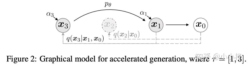
那么生成过程也可以用这个子序列的反向马尔卡夫链来替代，由于$S$ 以设置比原来的步数$L$ 小，那么就可以加速生成过程。这里的生成过程变成：

${\mathbf{x}}_{{\tau }_{i-1}}=\sqrt{{\alpha }_{{\tau }_{i-1}}}(\frac{{\mathbf{x}}_{{\tau }_i}-\sqrt{1-{\alpha }_{{\tau }_i}}{ϵ}_{\theta }({\mathbf{x}}_{{\tau }_i},{\tau }_i)}{\sqrt{{\alpha }_{{\tau }_i}}})+\sqrt{1-{\alpha }_{{\tau }_{i-1}}-{\sigma }_{{\tau }_i}^2}\cdot {ϵ}_{\theta }({\mathbf{x}}_{{\tau }_i},{\tau }_i)+{\sigma }_{{\tau }_i}ϵ$

其实上述的加速，我们是将前向过程按如下方式进行了分解：

$q_{\sigma ,\tau }({\mathbf{x}}_{1:T}|{\mathbf{x}}_0)=q_{\sigma ,\tau }({\mathbf{x}}_T|{\mathbf{x}}_0)\prod _{i=1}^S{q}_{\sigma }({\mathbf{x}}_{{\tau }_{i-1}}|{\mathbf{x}}_{{\tau }_i},{\mathbf{x}}_0)\prod _{t\in \overline{\tau }}{q}_{\sigma ,\tau }({\mathbf{x}}_t|{\mathbf{x}}_0)$

其中$\overline{\tau }=\{1,...,T\}\mathrm{\setminus }\tau$。这包含了两个图：其中一个就是由$\{{\mathbf{x}}_{{\tau }_i}{\}}_{i=1}^S$ 成的马尔可夫链，另外一个是剩余的变量$\{{\mathbf{x}}_t{\}}_{t\in \overline{\tau }}$ 成的星状图。同时生成过程，我们也只用马尔可夫链的那部分来生成：

$p_{\theta }({\mathbf{x}}_{0:T})=p({\mathbf{x}}_T)\underset{\text{use to produce sample}}{\underbrace{\prod _{i=1}^S{p}_{\theta }({\mathbf{x}}_{{\tau }_{i-1}}|{\mathbf{x}}_{{\tau }_i})}}\times \underset{\text{only for VLB}}{\underbrace{\prod _{t\in \overline{\tau }}{p}_{\theta }({\mathbf{x}}_0|{\mathbf{x}}_t)}}$

论文共设计了两种方法来采样子序列，分别是：

• Linear：采用线性的序列${\tau }_i=\lfloor ci\rfloor$；
• Quadratic：采样二次方的序列${\tau }_i=\lfloor c{i}^2\rfloor$；

这里的$c$ 一个定值，它的设定使得${\tau }_{-1}$ 接近$T$。论文中只对CIFAR10数据集采用Quadratic序列，其它数据集均采用Linear序列。

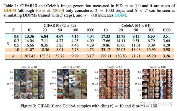
实验结果

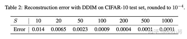
下表为不同的$\eta$ 以及不同采样步数下的对比结果，可以看到DDIM（$\eta =0$）在较短的步数下就能得到比较好的效果，媲美DDPM（$\eta =1$）的生成效果。如果$S$ 置为50，那么相比原来的生成过程就可以加速20倍。

代码实现

DDIM和DDPM的训练过程一样，所以可以直接在DDPM的基础上加一个新的生成方法（这里主要参考了https://github.com/ermongroup/ddim (opens new window)以及https://github.com/huggingface/diffusers/blob/main/src/diffusers/schedulers/scheduling_ddim.py (opens new window)），具体代码如下所示：

class GaussianDiffusion:
    def __init__(self, timesteps=1000, beta_schedule='linear'):
     pass

    # ...
        
 # use ddim to sample
    @torch.no_grad()
    def ddim_sample(
        self,
        model,
        image_size,
        batch_size=8,
        channels=3,
        ddim_timesteps=50,
        ddim_discr_method="uniform",
        ddim_eta=0.0,
        clip_denoised=True):
        # make ddim timestep sequence
        if ddim_discr_method == 'uniform':
            c = self.timesteps // ddim_timesteps
            ddim_timestep_seq = np.asarray(list(range(0, self.timesteps, c)))
        elif ddim_discr_method == 'quad':
            ddim_timestep_seq = (
                (np.linspace(0, np.sqrt(self.timesteps * .8), ddim_timesteps)) ** 2
            ).astype(int)
        else:
            raise NotImplementedError(f'There is no ddim discretization method called "{ddim_discr_method}"')
        # add one to get the final alpha values right (the ones from first scale to data during sampling)
        ddim_timestep_seq = ddim_timestep_seq + 1
        # previous sequence
        ddim_timestep_prev_seq = np.append(np.array([0]), ddim_timestep_seq[:-1])
        
        device = next(model.parameters()).device
        # start from pure noise (for each example in the batch)
        sample_img = torch.randn((batch_size, channels, image_size, image_size), device=device)
        for i in tqdm(reversed(range(0, ddim_timesteps)), desc='sampling loop time step', total=ddim_timesteps):
            t = torch.full((batch_size,), ddim_timestep_seq[i], device=device, dtype=torch.long)
            prev_t = torch.full((batch_size,), ddim_timestep_prev_seq[i], device=device, dtype=torch.long)
            
            # 1. get current and previous alpha_cumprod
            alpha_cumprod_t = self._extract(self.alphas_cumprod, t, sample_img.shape)
            alpha_cumprod_t_prev = self._extract(self.alphas_cumprod, prev_t, sample_img.shape)
    
            # 2. predict noise using model
            pred_noise = model(sample_img, t)
            
            # 3. get the predicted x_0
            pred_x0 = (sample_img - torch.sqrt((1. - alpha_cumprod_t)) * pred_noise) / torch.sqrt(alpha_cumprod_t)
            if clip_denoised:
                pred_x0 = torch.clamp(pred_x0, min=-1., max=1.)
            
            # 4. compute variance: "sigma_t(η)" -> see formula (16)
            # σ_t = sqrt((1 − α_t−1)/(1 − α_t)) * sqrt(1 − α_t/α_t−1)
            sigmas_t = ddim_eta * torch.sqrt(
                (1 - alpha_cumprod_t_prev) / (1 - alpha_cumprod_t) * (1 - alpha_cumprod_t / alpha_cumprod_t_prev))
            
            # 5. compute "direction pointing to x_t" of formula (12)
            pred_dir_xt = torch.sqrt(1 - alpha_cumprod_t_prev - sigmas_t**2) * pred_noise
            
            # 6. compute x_{t-1} of formula (12)
            x_prev = torch.sqrt(alpha_cumprod_t_prev) * pred_x0 + pred_dir_xt + sigmas_t * torch.randn_like(sample_img)

            sample_img = x_prev
            
        return sample_img.cpu().numpy()

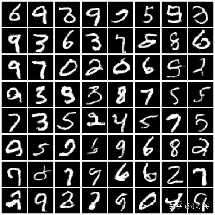
这里以MNIST数据集为例，训练的扩散步数为500，直接采用DDPM（即推理500次）生成的样本如下所示：

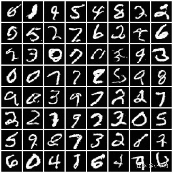
同样的模型，我们采用DDIM来加速生成过程，这里DDIM的采样步数为50，其生成的样本质量和500步的DDPM相当：

完整的代码示例见https://github.com/xiaohu2015/nngen (opens new window)。

其它：重建和插值

在DDIM论文中，还额外讨论了两个小点的内容**：重建和插值**。所谓重建是指的首先用原始图像求逆得到对应的噪音然后再进行生成的过程；而插值是指的对两个随机噪音进行插值从而得到融合两种噪音的图像。 首先是重建，对于DDIM，其$\eta =0$，这个时候从${\mathbf{x}}_t$ 成${\mathbf{x}}_{t-1}$ 更新公式就变为：

${\mathbf{x}}_{t-1}=\sqrt{{\alpha }_{t-1}}(\frac{{\mathbf{x}}_t-\sqrt{1-{\alpha }_t}{ϵ}_{\theta }({\mathbf{x}}_t,t)}{\sqrt{{\alpha }_t}})+\sqrt{1-{\alpha }_{t-1}}\cdot {ϵ}_{\theta }({\mathbf{x}}_t,t)$

我们进一步对上述公式进行变换可得到：

$\frac{{\mathbf{x}}_{t-1}}{\sqrt{{\alpha }_{t-1}}}=\frac{{\mathbf{x}}_t}{\sqrt{{\alpha }_t}}+(\sqrt{\frac{1-{\alpha }_{t-1}}{{\alpha }_{t-1}}}-\sqrt{\frac{1-{\alpha }_t}{{\alpha }_t}}){ϵ}_{\theta }({\mathbf{x}}_t,t)$

当$T$ 够大时，以上公式其实可以看成用欧拉法来求解一个常微分方程（ODE，ordinary differential equation）：

$\frac{{\mathbf{x}}_{t-\mathrm{\Delta }t}}{\sqrt{{\alpha }_{t-\mathrm{\Delta }t}}}=\frac{{\mathbf{x}}_t}{\sqrt{{\alpha }_t}}+(\sqrt{\frac{1-{\alpha }_{t-\mathrm{\Delta }t}}{{\alpha }_{t-\mathrm{\Delta }t}}}-\sqrt{\frac{1-{\alpha }_t}{{\alpha }_t}}){ϵ}_{\theta }({\mathbf{x}}_t,t)$

这里令$\sigma =\sqrt{1-\alpha }/\sqrt{\alpha }$，$\overline{\mathbf{x}}=\mathbf{x}/\sqrt{\alpha }$，它们都是关于$t$ 函数，这样对应的ODE就是：

$\text{d}\overline{\mathbf{x}}(t)={ϵ}_{\theta }(\frac{\overline{\mathbf{x}}(t)}{\sqrt{{\sigma }^2+1}},t)\text{d}\sigma (t)$

看成ODE后，我们可以利用如下公式对生成过程进行逆操作：

$\frac{{\mathbf{x}}_{t+1}}{\sqrt{{\alpha }_{t+1}}}=\frac{{\mathbf{x}}_t}{\sqrt{{\alpha }_t}}+(\sqrt{\frac{1-{\alpha }_{t+1}}{{\alpha }_{t+1}}}-\sqrt{\frac{1-{\alpha }_t}{{\alpha }_t}}){ϵ}_{\theta }({\mathbf{x}}_t,t)$

这意味着，我们可以由一个原始图像${\mathbf{x}}_0$ 到对应的随机噪音${\mathbf{x}}_T$，然后我们再用${\mathbf{x}}_T$ 行生成就可以重建原始图像${\mathbf{x}}_0$(具体的代码实现见https://github.com/openai/improved-diffusion/blob/main/improved_diffusion/gaussian_diffusion.py#L524-L560 (opens new window)）。论文也通过在CIFAR10测试集上的实验来证明当步数足够时，这种方式可以得到较低的重建误差：

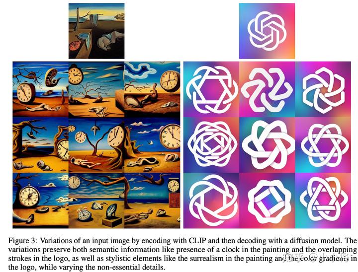
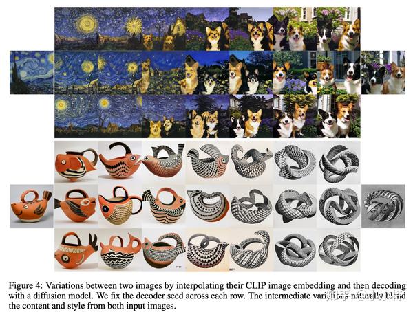
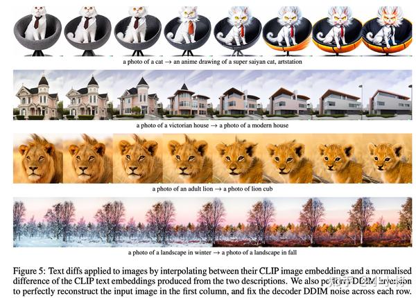
第二个插值，对于DDIM，两个不同的随机噪音会产生不同的图像，但是如果我们对这两个随机噪音进行插值生成新的${\mathbf{x}}_T$，那么将生成融合的图像。这里采用的插值方法是球面线性插值（ spherical linear interpolation）：

${\mathbf{x}}_T^{(\alpha )}=\frac{\sin ((1-\alpha )\theta )}{\sin (\theta )}{\mathbf{x}}_T^{(0)}+\frac{\sin (\alpha \theta )}{\sin (\theta )}{\mathbf{x}}_T^{(1)}\theta =\arccos (\frac{({\mathbf{x}}_T^{(0)}{)}^{\text{T}}{\mathbf{x}}_T^{(1)}}{\parallel {\mathbf{x}}_T^{(0)}\parallel \parallel {\mathbf{x}}_T^{(1)}\parallel })$

这里的参数$\alpha \in [0,1]$ 制插值系数，具体的代码实现见https://github.com/ermongroup/ddim/blob/main/runners/diffusion.py#L296-L334 (opens new window)。下图展示了一些具体的插值效果：

DDIM的重建和插值也在文本转图像模型DALLE-2中使用，不过这里插值的是扩散模型的条件CLIP image embedding，详情见论文**https://arxiv.org/abs/2204.06125 (opens new window)**。

小结

如果从直观上看，DDIM的加速方式非常简单，直接采样一个子序列，其实论文https://arxiv.org/abs/2102.09672 (opens new window)也采用了类似的方式来加速。另外DDIM和其它扩散模型的一个较大的区别是其生成过程是确定性的。

参考

• https://arxiv.org/abs/2010.02502 (opens new window)
• https://github.com/ermongroup/ddim (opens new window)
• https://github.com/openai/improved-diffusion (opens new window)
• https://github.com/huggingface/diffusers/blob/main/src/diffusers/schedulers/scheduling_ddim.py (opens new window)
• https://github.com/CompVis/latent-diffusion/blob/main/ldm/models/diffusion/ddim.py (opens new window)
• https://kexue.fm/archives/9181 (opens new window)